Choice Models and its Applications
Welcome to the course!
How to use these slides
These slides leverage Quarto, an open-source scientific and technical publishing system from Posit (formerly RStudio):
- Create dynamic content with Python, R, Julia, and Observable
- Publish reproducible, production quality articles, presentations, dashboards, websites, blogs, and books in HTML, PDF, MS Word, ePub, and more
- Write using Pandoc markdown, including equations, citations, crossrefs, figure panels, callouts, advanced layout, and more.
For our course, we’ll use the following notation:
- Link will be colored in dark-orange
- Inline equations and variables will be rendered in
gray - Code chunks will be provided along with outputs (in
Python)
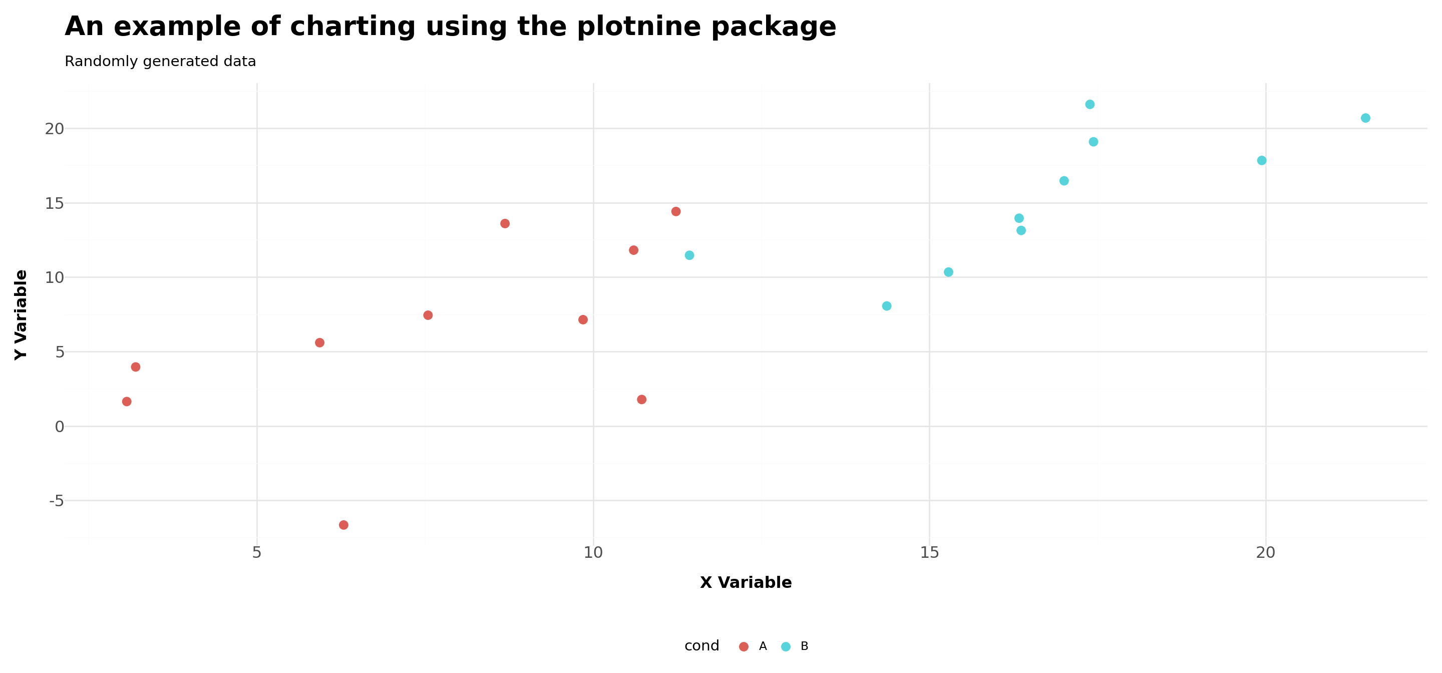
An example of a code chunk
# Generating data
np.random.seed(0)

dat = pd.DataFrame({
    'cond': np.repeat(['A', 'B'], 10),
    'xvar': np.arange(1, 21) + np.random.normal(0, 3, 20),
    'yvar': np.arange(1, 21) + np.random.normal(0, 3, 20)
})

dat=tp.as_tibble(dat)

theme_plots= theme(
  legend_position='bottom',
  axis_title=element_text(face='bold',size=10),
  plot_title=element_text(face='bold',size=15)
  )

# Plotting
Plot=(

  ggplot(dat,aes(x='xvar',y='yvar',fill='cond',color='cond'))+
              geom_point()+
              labs(
              title = 'An example of charting using the plotnine package',
              subtitle = 'Randomly generated data',
              x = 'X Variable',
              y = 'Y Variable')
            + scale_y_continuous(breaks = range(-10,25,5))
            + scale_x_continuous(breaks = range(-10,25,5))
            + theme_minimal()
            + theme(
              legend_position='bottom',
              axis_title=element_text(face='bold',size=12),
              axis_text=element_text(size=12),
              plot_title=element_text(face='bold',size=20),
              figure_size=(15,7)
              )
)

Plot.show()
Course Outline
The first section of the Quantitative Marketing course will cover choice models:
- Binary Response Models: Logit/Probit
- Multi-choice Models: Multinomial Logit
- Economic Implications of multi-choice models
- Market-basket Analysis and further topics on choice models
To the best of our capabilities, we will stick to a hands-on approach, focusing on practical applications and using the economic/econometric tools and concepts you’ve learned so far to interpret our findings
Handouts
To maintain reproducibility, at the end of each class, a handout containing all the coding steps with detailed explanations will be provided. As such, students can download the file and replicate all the contents from each lecture on their end.
Bibliography and References
Although emphasis will be given to the practical aspects (i.e, coding) around the subjects, it is expected that students are well-versed in statistics/econometrics
For a detailed discussion around the methodological approaches discussed throughout the lectures, you can refer to the following textbooks (graduate-level):
- Discrete Choice Methods with Simulation - (Train 2009)
- Econometric Analysis - (Greene 2011)
- Econometrics - (Hayashi 2000)
For a broader discussion around the practical applications on Marketing topics, we’ll follow (Chapman and Feit 2015)
\(\rightarrow\) For those that want to extend their knowledge beyond the topics covered in the lectures, the professor will provide a range of academic papers, as well as policy/whitepapers that cover further topics on Quantitative Marketing
Introduction to Discrete Choice Models
Marketing practitioners are often concerned about consumers decisions around a defined set of choices:
Consumers choose between a binary decision of buy/not buy, given product, consumer, and environmental characteristics
Faced with a defined set of products, make a decision around which products to buy
After experiencing a flow of consumption from a product or service up to time \(t\), decide whether to continue consumption at \(\small t+1\) or churn
Eliciting knowledge about individual choices shed light on consumer preferences and help marketers to understand how consumers value certain product attributes
Aggregating individual choices helps marketers understand how the demand curve for a given product or industry works
Binary Choice Models
- Motivation: among a defined set of two mutually exclusive alternatives, consumers make a decision by choosing one alternative in spite of the other:
\[ \small Y_i=\begin{cases} 1, & \text{if $Y_i$ = a predefined alternative}\\ 0, & \text{otherwise} \end{cases} \]
- These models implicitly tell about consumer’s preferences regarding several consumption decisions. Say that we know that a set \(X\) of characteristics (which may be consumer-specific, environmental, or product) affect \(i\)’s decision. We can then model such decision by:
\[ \small Y_i=f(X_i) \]
- Our starting point will be to define what \(f(X)\) should look like. Depending on the shape of this function, the interpretation becomes a probabilistic measurement
Binary Choice Models - Churn
- One of the most widely applicable areas of binary choice modeling refers to churn modeling:
Definition
Churn refers to the the % of customers who discontinue their use of a business’s products or services over a certain time period. This concept is important for businesses because it affects their revenue and offers insights into customer satisfaction and loyalty:
A high churn rate may suggest there are issues with the product, service, or overall customer experience
A low churn rate may suggest the existence of customer loyalty, high switching costs, or valuable attributes from the offer
Churn modeling offers valuable insights to marketers as it is possible to derive actions ex-ante its occurrence and prevent customers from churning
This issue becomes more relevant when customer acquisition costs increase
Hands-On Exercise
Description
- You work as a quantitative analyst at a big regional bank and just got access to the bank’s Customer Relationship Manager (CRM) data, comprising a sample of 10,000 bank customers and its actual engagement status (whether or not he/she has churned) over the study period. Your manager wants you to use this data and investigate the following points:
- What is the percentage of customers that are churning during the study period?
- What are the key aspects that drove historical churn?
- Which action plans would you recommend so as to preemptively identify and avoid future churn from customers?
- You can download the
bank-dataset.csvdata using the Download button below
Note: this dataset is be primarily based on this Kaggle notebook, although some adaptations have been made for teaching purposes
Before we start: tech-setup
- To install all necessary
Pythonlibraries, use the terminal to install and thenimportall packages inside a notebook. First, install all dependencies by downloading therequirements.txtfile and running the following script on your terminal:
- After you have everything properly installed, it is time to load the packages in your session - make sure to load this at the beginning of your script/notebook:
Tech-setup
In the official page (link here) of our course, I have outlined a few steps for you to get started using Python and install all dependencies that we will be using.
Variable Descriptives
- To begin our investigation, let’s do a simple variable description of the variables that we have in our dataset:
| Summary Statistics | |||||||||
|---|---|---|---|---|---|---|---|---|---|
| credit_score | age | tenure | balance | products_number | credit_card | active_member | estimated_salary | churn | |
| count | 10,000 | 10,000 | 10,000 | $10,000 | 10,000.00 | 10,000.00 | 10,000.00 | $10,000 | 10,000.00 |
| mean | 651 | 39 | 5 | $76 | 1.53 | 0.71 | 0.52 | $100 | 0.20 |
| std | 97 | 10 | 3 | $62 | 0.58 | 0.46 | 0.50 | $58 | 0.40 |
| min | 350 | 18 | 0 | $0 | 1.00 | 0.00 | 0.00 | $0 | 0.00 |
| 25% | 584 | 32 | 3 | $0 | 1.00 | 0.00 | 0.00 | $51 | 0.00 |
| 50% | 652 | 37 | 5 | $97 | 1.00 | 1.00 | 1.00 | $100 | 0.00 |
| 75% | 718 | 44 | 7 | $128 | 2.00 | 1.00 | 1.00 | $149 | 0.00 |
| max | 850 | 92 | 10 | $251 | 4.00 | 1.00 | 1.00 | $200 | 1.00 |
# Read the CSV file into a pandas DataFrame
Data = pd.read_csv('Assets/bank-dataset.csv')
Summary = Data.drop('customer_id',axis=1).describe().reset_index()

# Print the structure of the DataFrame
Table = (
  GT(Summary)
  .cols_align('center')
  .tab_header(title=md("**Summary Statistics**"))
  .tab_stub('index')
  .fmt_number(columns=['credit_score','age','tenure'],decimals = 0)
  .fmt_number(columns=['products_number','credit_card','active_member','churn'],decimals = 2)
  .fmt_currency(columns=['balance','estimated_salary'],decimals=0)
  .opt_stylize(style=1,color='red')
)

#Output
Table.tab_options(table_width="100%",table_font_size="25px")
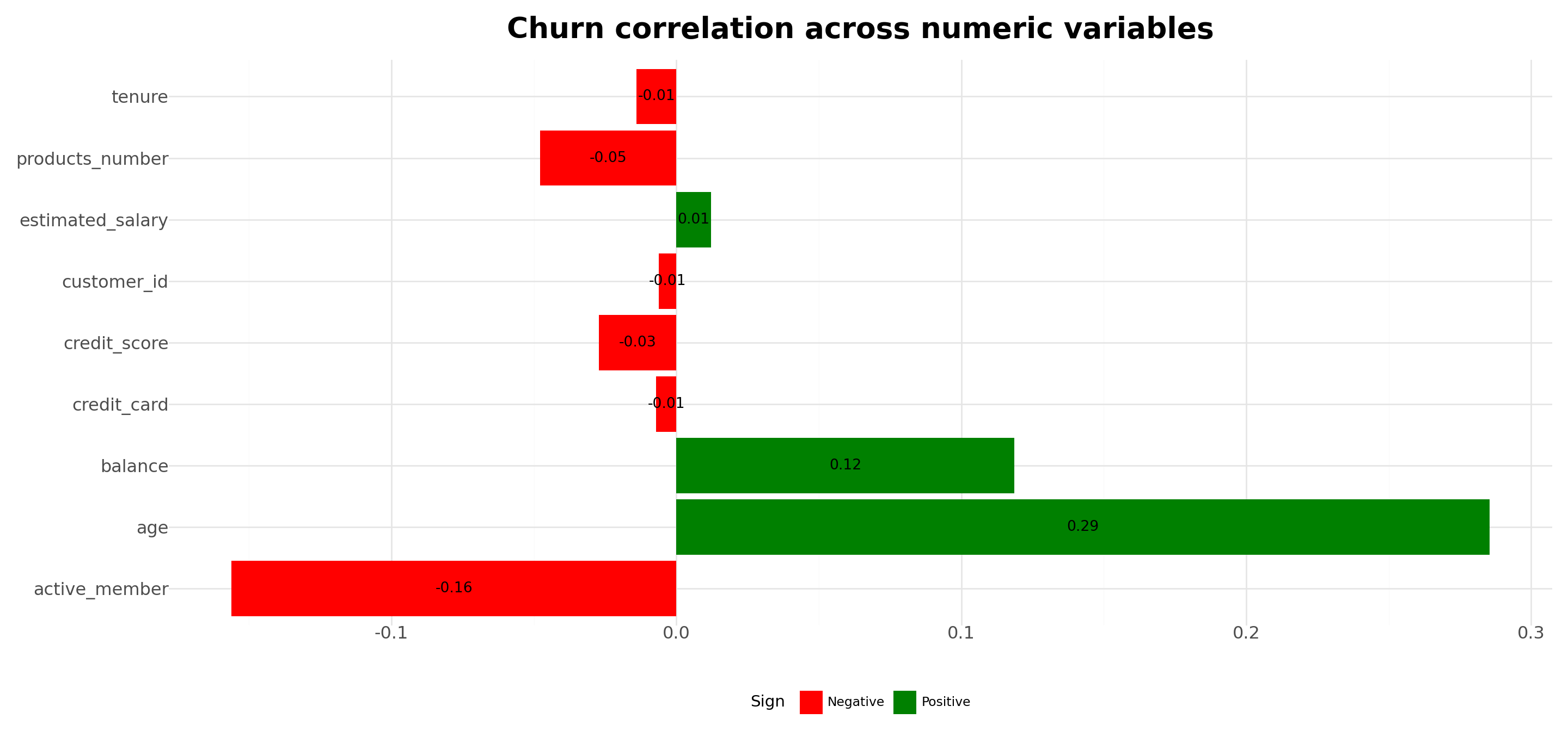
Analyzing churn correlation with customer characteristics
# Select numeric columns and calculate correlation with churn
correlation_df = (
  Data
  .select_dtypes(include='number')
  .corr()
  .iloc[:-1, -1]
  .reset_index()
)

# Rename columns
correlation_df.columns = ['Variable', 'Correlation']

# Add 'Sign' column based on correlation values
correlation_df['Sign'] = correlation_df['Correlation'].apply(lambda x: 'Positive' if x > 0 else 'Negative')

#Chart
Plot = (
  ggplot(correlation_df, aes(x='Variable', y='Correlation', fill='Sign'))+
  geom_col()+
  geom_text(aes(label=correlation_df['Correlation'].round(2)),size=10, color='black',position=position_stack(vjust=0.5))+  # Add annotations
  scale_fill_manual(values=['red','green'])+
  coord_flip()+
  labs(title='Churn correlation across numeric variables')+
  theme_minimal()+
  theme(
    legend_position='bottom',
    axis_title=element_blank(),
    axis_text=element_text(size=12),
    plot_title=element_text(face='bold',size=20),
    figure_size=(15,7)
    )
)

#Display Output
Plot.show()
Modeling Discrete Choice Models
- Say that we are interested in modeling the occurrence of
churn, which is a discrete variable for each customer \(i\):
\[ Y_i= \begin{cases} 1, \text{if the customer has churned}\\ 0, \text{if the customer is still an active client} \end{cases} \]
- If we have a set of covariates, \(X_i\), then we can define the relationship:
\[ Y_i=f(X_i) \]
- How our \(f(X_i)\) should look like?
- What is the interpretation of the estimates that we’ll find?
Linear Probability Models (LPM)
- The simplest approach that we can take is to assume that \(Y\) is linear on the set of characteristics \(X\). In other words, \(f(X)\) is a linear model:
\[ Y_i= P(Y_i=1|X_i)=\alpha + \beta_1x_1+\beta_2x_2+...+\beta_nx_n+\varepsilon_i \]
We can then use Ordinary Least Squares (OLS) to model such relationship. Because the functional form of \(f(X)\) is assumed to be linear, we call this a linear probability model (LPM):
Because the relationship between \(Y\) and \(X\) is assumed to be linear, the changes in the probability (or likelihood) of
churnare linear on the parameters \(\beta\). For example, for \(x_1\):
\[ \dfrac{\partial Y}{\partial x_1}=\beta_1 \]
Is the LPM a biased estimator?
- If the OLS assumptions are valid, \(\beta_{OLS}\) is still a consistent estimator of the population average relationship between \(Y\) and \(X\), regardless of the type of dependent variable:
\[ \begin{align} & \beta_{OLS}=(X'X)^{-1}X'Y\\ & \beta_{OLS}=(X'X)^{-1}X'(X\beta+\epsilon)=\underbrace{(X'X)^{-1}(X'X)}_{I}\beta+(X'X)^{-1}X'\epsilon\\ & \beta_{OLS}=\beta + (X'X)^{-1}X'\epsilon \end{align} \]
- If we assume that \(X\perp\epsilon\) - i.e, no ommited variables-, we see that \(\beta_{OLS}\) is an unbiased estimator of the average effect of \(X\) on \(Y\):
\[ \text{if } X\perp\epsilon \rightarrow \beta_{OLS}=\beta + (X'X)^{-1}\underbrace{X'\epsilon}_{=0}\rightarrow \beta_{OLS}=\beta \]
Modeling churn via LPM
- Suppose we want to understand the determinants of customer’s churn over time. For that, we’ll consider the following variables:
\[ \text{if } X=\begin{bmatrix} CreditScore \\ D(Gender) \\ Age \\ Tenure \\ Balance \\ \#Products \\ D(CreditCard) \\ D(Active) \\ Salary \end{bmatrix} \rightarrow Y \sim X'\beta+\epsilon \]
LPM Estimation
                            OLS Regression Results
==============================================================================
Dep. Variable:                  churn   R-squared:                       0.136
Model:                            OLS   Adj. R-squared:                  0.135
Method:                 Least Squares   F-statistic:                     174.6
Date:                Fri, 04 Apr 2025   Prob (F-statistic):          8.76e-309
Time:                        13:05:07   Log-Likelihood:                -4364.5
No. Observations:               10000   AIC:                             8749.
Df Residuals:                    9990   BIC:                             8821.
Df Model:                           9
Covariance Type:            nonrobust
====================================================================================
                       coef    std err          t      P>|t|      [0.025      0.975]
------------------------------------------------------------------------------------
const               -0.1025      0.034     -3.027      0.002      -0.169      -0.036
credit_score     -9.264e-05   3.88e-05     -2.389      0.017      -0.000   -1.66e-05
gender_Male         -0.0773      0.008    -10.267      0.000      -0.092      -0.063
age                  0.0113      0.000     31.505      0.000       0.011       0.012
tenure              -0.0018      0.001     -1.426      0.154      -0.004       0.001
balance              0.0007   6.31e-05     11.003      0.000       0.001       0.001
products_number     -0.0043      0.007     -0.630      0.529      -0.018       0.009
credit_card         -0.0030      0.008     -0.360      0.719      -0.019       0.013
active_member       -0.1432      0.008    -19.016      0.000      -0.158      -0.128
estimated_salary  7.118e-05   6.52e-05      1.092      0.275   -5.66e-05       0.000
==============================================================================
Omnibus:                     1513.285   Durbin-Watson:                   1.994
Prob(Omnibus):                  0.000   Jarque-Bera (JB):             2319.357
Skew:                           1.176   Prob(JB):                         0.00
Kurtosis:                       3.176   Cond. No.                     6.09e+03
==============================================================================

Notes:
[1] Standard Errors assume that the covariance matrix of the errors is correctly specified.
[2] The condition number is large, 6.09e+03. This might indicate that there are
strong multicollinearity or other numerical problems.
# Read the CSV file into a pandas DataFrame
Data = pd.read_csv('Assets/bank-dataset.csv')
# Convert 'gender' into dummy variables
Data = pd.get_dummies(Data, columns=['gender'], drop_first=True)
# Define independent and dependent variables
X = Data[['credit_score', 'gender_Male', 'age', 'tenure', 'balance', 'products_number', 'credit_card', 'active_member', 'estimated_salary']]
y = Data['churn']
# Add a constant to the independent variables matrix for the intercept
X = sm.add_constant(X)
# Fit the linear regression model
model = sm.OLS(y, X.astype(float)).fit()
# Print the regression summary
print(model.summary())Overall analysis
- All else equal, an additional year increases the likelihood of churning by:
\[ \partial Y/\partial Age=\beta_{Age}\approx 0.0113 \]
- Moving from the \(25^{th}\) to the \(75^{th}\) percentile of
ageincreases the likelihood by \(\beta_{Age}\times IQR(Age)=(44-32)\times 0.0113 \approx 14\) or 14%
- Male customers tend to churn, on average, \(7.7\%\) less than Female customers:
\[ \partial Y/\partial D(genderMale)=\beta_{genderMale}\approx =-0.078 \]
- Similar analyses can be made for the following continuous variables (see Code in next slide)
Analyses
| Summary Statistics | |||
|---|---|---|---|
| Change in Covariate | Coefficient from OLS | Change on Outcome (in %) | |
| credit_score | 134 | −0.0001 | −1.24% |
| age | 12 | 0.0113 | 13.57% |
| tenure | 4 | −0.0018 | −0.74% |
| balance | 128 | 0.0007 | 8.86% |
| products_number | 1 | −0.0043 | −0.43% |
| estimated_salary | 98 | 0.0001 | 0.70% |
| gender_Male | 1 | −0.0773 | −7.73% |
| credit_card | 1 | −0.0030 | −0.30% |
| active_member | 1 | −0.1432 | −14.32% |
# Define continuous and dummy variables
continuous_vars = ['credit_score', 'age', 'tenure', 'balance', 'products_number', 'estimated_salary']
dummy_vars = ['gender_Male', 'credit_card', 'active_member']

# Get coefficient estimates from the model
estimates = model.params.reset_index()
estimates.columns = ['Variable', 'estimate']

# Calculate IQR for continuous variables
iqr_df = Data[continuous_vars].apply(lambda x: x.quantile(0.75) - x.quantile(0.25), axis=0)
iqr_df = pd.DataFrame({'Variable': iqr_df.index, 'Change': iqr_df.values})

# Create a DataFrame for dummy variables
dummy_df = pd.DataFrame({'Variable': dummy_vars, 'Change': 1})

# Combine continuous and dummy variable dataframes
combined_df = pd.concat([iqr_df, dummy_df])

# Merge with coefficient estimates
result_df = pd.merge(combined_df, estimates, on='Variable', how='left')

# Calculate partial changes
result_df['partial_change'] = (result_df['Change'] * result_df['estimate'])

#Table
Table= (
  GT(result_df)
  .cols_align('center')
  .tab_stub(rowname_col='Variable')
  .cols_label(
    Change = 'Change in Covariate',
    estimate = 'Coefficient from OLS',
    partial_change = 'Change on Outcome (in %)'
    )
  .fmt_number(columns = 'Change',decimals=0)
  .fmt_number(columns = 'estimate',decimals=4)
  .fmt_percent(columns='partial_change',decimals=2)
  .tab_header(title=md("**Summary Statistics**"))
  .opt_stylize(style=1,color='red')
)

Table.tab_options(table_width="100%",table_font_size="25px")
Limitations of the LPM
- Although a consistent estimator of the average effect, the LPM has limitations when it comes to its practical implications to binary outcomes:
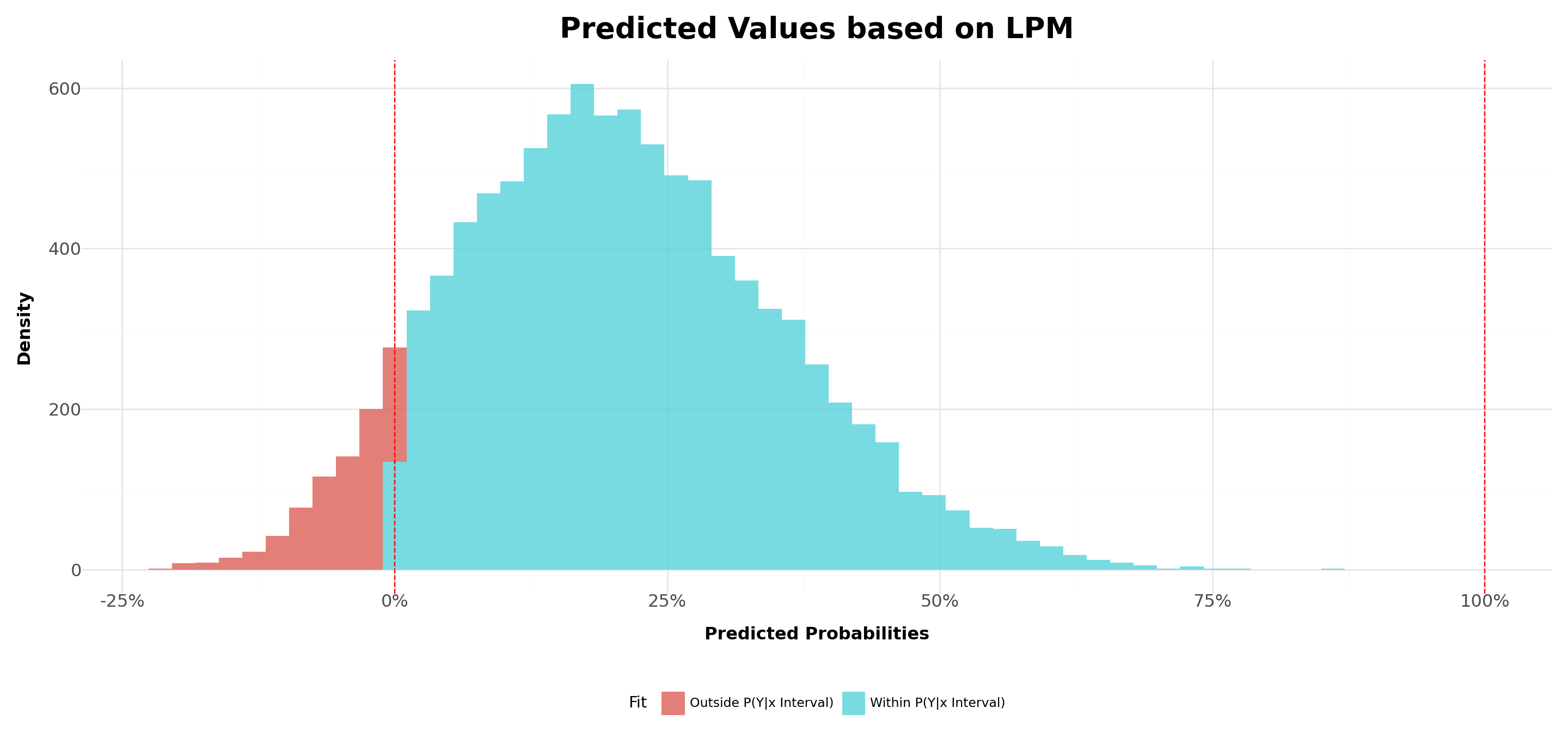
Churn probabilities should lie within \([0,1]\), but the predicted probabilities, \(\hat{Y}\), have continuous support \((-\infty,+\infty)\). When the goal is to predict outcomes, this creates probabilities that are outside of the ranges
There is an implicit assumption that the effects are linear, which may not hold true. Example, an increase of $1,000 in customer’s income may have significant impacts on churn likelihood when customers are from the bottom of the income distribution, but the effects should dampen as we move towards the top of the income distribution
Heteroskedasticity
\(R^2\) is not well-defined
Limitations of the LPM
- Even though we can achieve consistent estimators, we’ll have heteroskedasticity in our estimates by construction. To see that, recall that the conditional expectation of Y given X is given by:
\[ \small E(Y|X)=\underbrace{[P(Y=1|X]}_{X\beta\times 1} + \underbrace{[1-P(Y=1|X)]\times 0}_{=0} = X\beta \]
- Given that the variance of a Bernoulli Distribution is given by \(p \times (1-p)\), then:
\[ V(Y|X)=P(Y|X)\times[1-P(Y|X)]=X\beta\times(1-X\beta) \text{, which clearly depends on } X \]
- In most linear probability models, \(R^2\) has no meaningful interpretation:
- Regression line can never fit the data perfectly if the dependent variable is binary and the regressors are continuous
- Since LPM predicts probabilities, the dependent variable is binary (\(0\) or \(1\)), making the interpretation of \(R^2\) problematic. The model often produces predicted values outside the \([0,1]\) range, leading to unreliable goodness-of-fit assessments
Introducing non-linear binary models
Recall that the limitations of the LPM stem from the fact that \(f(X)=X'\beta\). It might be that a linear relationship does not capture all aspects that a churn analysis should have!
To that point, we need to think about a new relationship, \(Y=f(X)\), that fulfills the following points:
- The predicted outcomes, \(\hat{Y}\), lie between 0 and 1
- The effects do not need to be linear on the parameters
- Ideally, we’d want to apply a non-linear transformation in such a way that the relationship between Y and X is sigmoid (or S-shaped) curve: the changes in the predicted probability tend to go to zero as we approach the lower and upper bounds of the distribution of X
- The most known cases are logistic regression (\(f(x)=\Lambda (x)\)) and Probit (\(f(x)=\Phi(X)\))
Logistic Regression
Like any other transformation function, the idea behind using \(\Lambda(X)\) lies on the latent variable approach: think about an unobserved component, \(Y^\star\), which is a continuous variable, such as how much a consumer values a product.
Although we do not observe \(Y^\star\), we do observe the consumer’s decision of buying or not buying the product, depending on a given threshold:
\[ Y= \begin{cases} 1, \text{ if }Y^\star>0\\ 0, \text{ if }Y^\star\leq0\\ \end{cases} \]
- Therefore, we can see that the probability of buying depends on a latent variable, which is not observed by the econometrician:
\[ P(Y=1|X)=P(Y^\star>0|X)=P(\underbrace{X\beta+\varepsilon}_{Y^{\star}}>0|X) \]
Logistic Regression, continued
- We can rearrange terms and find that:
\[ P(Y=1|X)=P(\underbrace{X\beta+\varepsilon}_{Y^{\star}}>0|X)\rightarrow \underbrace{P(\varepsilon>-X\beta|X)\equiv P(\varepsilon<X\beta|X)}_{\text{Under Simmetry}} \]
- Therefore, this framework can be used to think about any cumulative density function which has the simmetry property. For the case of Logistic Regression, our transformation function that maps \(Y^\star\) (how much consumer values a good) to \(Y\) (decision to buy or not buy) is:
\[ f(Y^\star)=\Lambda(Y^\star)=\dfrac{\exp(X\beta)}{1+\exp(X\beta)} \]
- Estimation is made using Maximum Likelihood estimators.
Applying Logistic Regression
Optimization terminated successfully.
         Current function value: 0.435323
         Iterations 6
Logit Regression Results
==============================================================================
Dep. Variable: churn No. Observations: 10000
Model: Logit Df Residuals: 9990
Method: MLE Df Model: 9
Date: Fri, 04 Apr 2025 Pseudo R-squ.: 0.1388
Time: 13:05:08 Log-Likelihood: -4353.2
converged: True LL-Null: -5054.9
Covariance Type: nonrobust LLR p-value: 1.475e-296
====================================================================================
coef std err z P>|z| [0.025 0.975]
------------------------------------------------------------------------------------
const -3.4761 0.241 -14.397 0.000 -3.949 -3.003
credit_score -0.0007 0.000 -2.349 0.019 -0.001 -0.000
gender_Male -0.5429 0.054 -10.060 0.000 -0.649 -0.437
age 0.0729 0.003 28.561 0.000 0.068 0.078
tenure -0.0147 0.009 -1.585 0.113 -0.033 0.003
balance 0.0050 0.000 10.964 0.000 0.004 0.006
products_number -0.0362 0.046 -0.780 0.436 -0.127 0.055
credit_card -0.0290 0.059 -0.493 0.622 -0.144 0.086
active_member -1.0793 0.057 -18.860 0.000 -1.191 -0.967
estimated_salary 0.0005 0.000 1.060 0.289 -0.000 0.001
====================================================================================# Read the CSV file into a pandas DataFrame
Data = pd.read_csv('Assets/bank-dataset.csv')
# Convert 'gender' into dummy variables
Data = pd.get_dummies(Data, columns=['gender'], drop_first=True)
# Define independent and dependent variables
X = Data[['credit_score', 'gender_Male', 'age', 'tenure', 'balance', 'products_number', 'credit_card', 'active_member', 'estimated_salary']]
y = Data['churn']
# Add a constant to the independent variables matrix for the intercept
X = sm.add_constant(X)
# Fit the linear regression model
model = sm.Logit(y, X.astype(float)).fit()
# Print the regression summary
print(model.summary())Logit Properties #1: probabilities within the [0,1] interval
- One interesting thing to note is that, due to the properties of \(\Lambda(\cdot)\), our estimated probabilities will fall within \([0,1]\) depending on \(X\):
- When \(X\rightarrow\infty\), the probability of buying in our example tends to 1:
\[ \Lambda(Y)=\dfrac{\exp(Y)}{1+\exp(Y)}=\dfrac{\exp(X\beta)}{1+\exp(X\beta)}\rightarrow1 \]
- On the other hand, when \(X\rightarrow -\infty\), the probability of buying in our example tends to 0:
\[ \Lambda(Y)=\dfrac{\exp(Y)}{1+\exp(Y)}=\dfrac{\exp(X\beta)}{1+\exp(X\beta)}\rightarrow \dfrac{0}{1}=0 \]
Logit Properties #2: the odds-ratio
- Recall that the logit estimation for \(\small P(Y|X)\) is given by:
\[ \small P(Y)=\dfrac{\exp(X\beta)}{1+\exp(X\beta)},\text{ which we will call by } p \]
- Looking at the inverse, \(1/p\), we can see that:
\[ \small \dfrac{1}{p}=\dfrac{1+\exp(X\beta)}{\exp(X\beta)}=1+\dfrac{1}{\exp{X\beta}}\rightarrow \dfrac{1-p}{p}=\dfrac{1}{\exp{X\beta}} \]
- Inverting and taking logs on both sides, we’ll have:
\[ \small \log{\bigg(\dfrac{p}{1-p}}\bigg)=X\beta=\alpha+\beta_1x_1+\beta_2x_2+...\beta_kx_k \]
Logit Properties #2: the odds-ratio (continued)
- Therefore, whenever we’re estimating a logit model, our transformation function, \(\Lambda(\cdot)\) is actually estimating \(\small \dfrac{p}{1-p}\):
\[ \small logit(p)=\alpha+\beta_1x_1+\beta_2x_2+...\beta_kx_k \]
The term \(\small \dfrac{p}{1-p}\) is called odds-ratio, and is simply the ratio of the probability of success over the probability of failure
Hence, if we want to recover the impacts of any change in the odds-ratio due to our covariates, we can exponentiate our coefficients:
\[ \small \text{if } \log\bigg(\dfrac{p}{1-p}\bigg)=\alpha+\beta_1x_1+\beta_2x_2+...\beta_kx_k\rightarrow \dfrac{p}{1-p}=\exp(\alpha+\beta_1x_1+\beta_2x_2+...\beta_kx_k) \]
Logit Properties #2: the odds-ratio (continued)
- In previous slides, we noted that the effect of
Genderis \(\small\beta_2=-0.54\). Holding everything fixed, the odds-ratio betweenGender=1(Male) versusGender=0(Female) is given by:
\[ \small \dfrac{p}{1-p}=\exp(\beta_2)=\exp(-0.54)\approx0.58 \]
Put another way, the chances of being a churned client are \(\small 0.58-1=-0.42\) or 42% less likely for men!
Similarly, if we look at
Age(\(\beta_3=0.07\)), one additional year increases churn probability by:
\[ \exp(\beta_1)=[\exp(0.0728688)-1]\approx 0.07 \text{ or } 7.55\% \]
| Summary Statistics | |||
|---|---|---|---|
| OddsRatio | Multiplier | ChangeOdds | |
| const | 3.09% | 1 | −96.91% |
| credit_score | 99.93% | 100 | −7.00% |
| gender_Male | 58.10% | 1 | −41.90% |
| age | 107.56% | 1 | 7.56% |
| tenure | 98.54% | 1 | −1.46% |
| balance | 100.51% | 10 | 5.10% |
| products_number | 96.45% | 1 | −3.55% |
| credit_card | 97.14% | 1 | −2.86% |
| active_member | 33.98% | 1 | −66.02% |
| estimated_salary | 100.05% | 100 | 5.00% |
# Calculate Odds Ratio and Change in Odds
odds_ratio = pd.DataFrame({
  'OddsRatio': model.params.apply(lambda x: round(np.exp(x), 4)),
  'Multiplier': [1, 100, 1, 1, 1, 10, 1, 1, 1, 100]
  })

odds_ratio = odds_ratio.reset_index()

odds_ratio['ChangeOdds'] = ((odds_ratio['OddsRatio'] - 1) * odds_ratio['Multiplier']).map(lambda x: f"{x:.2%}")

#Table
Table = (
  GT(odds_ratio)
  .cols_align('center')
  .tab_stub(rowname_col='index')
  .cols_label(
    OddsRatio = 'Odds Ratio',
    Multiplier = 'Multiplier',
    ChangeOdds = 'Change in Probality (in p.p)'
    )
  .fmt_number(columns = 'odds',decimals=0)
  .fmt_percent(columns=['OddsRatio','ChangeOdds'],decimals=2)
  .tab_header(title=md("**Summary Statistics**"))
  .opt_stylize(style=1,color='red')
)

Table.tab_options(table_width="100%",table_font_size="25px")
Logit Properties #3: different marginal effects
One of the caveats of LPM was that the marginal effect was constant, which does not make a lot of sense from a probabilistic sense
With Logit, the marginal effects are not equal to \(\beta\) anymore. To see that, take the derivative of \(P(Y|X)\) with respect to \(x_1\):
\[ \dfrac{\partial\Lambda(X\beta)}{\partial x_1}=\beta_1 \times\dfrac{\partial\Lambda(X\beta)}{\partial X\beta} \]
As we can see, the effects are not going to be linear anymore!
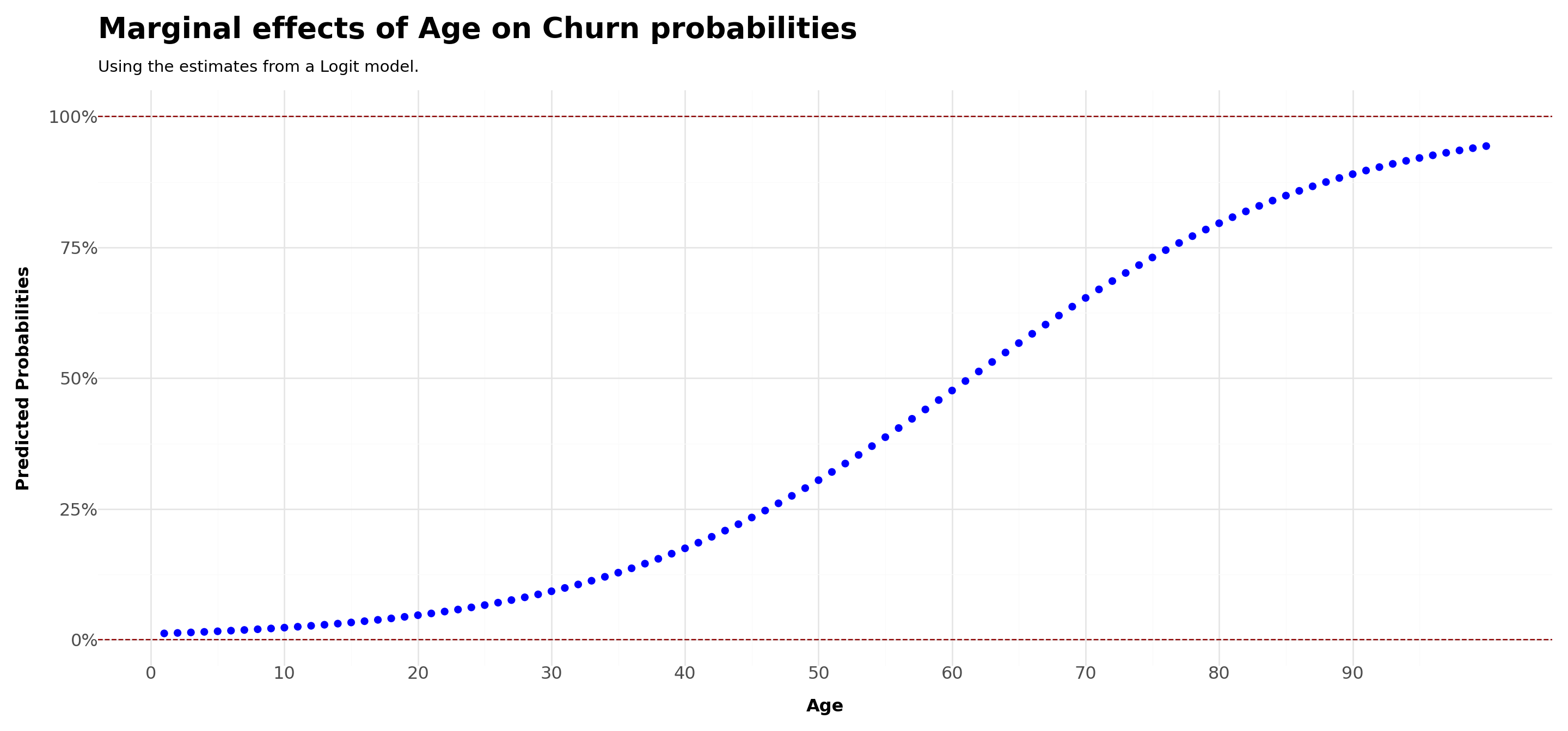
Put another way, given different levels of X, we may have different marginal effects on the probabilities - in what follows, we’ll analyze the case of
age
# Load data
data = pd.read_csv('Assets/bank-dataset.csv')
data['gender'] = np.where(data['gender'] == 'Male', 1, 0)

# Fit logistic regression model
X = data[['credit_score', 'gender', 'tenure', 'balance', 'products_number', 'credit_card', 'active_member', 'estimated_salary','age']]
X = sm.add_constant(X)  # Add constant term for intercept
y = data['churn']
model = sm.Logit(y, X).fit()

# Set all other variables to the mean
new_data = X.drop(columns=['age']).mean(numeric_only=True).to_frame().transpose()
new_data = pd.DataFrame(np.repeat(new_data.values, 100, axis=0),columns=new_data.columns)
age_df = pd.DataFrame(pd.Series(range(1, 101)), columns=['age'])

# Concatenate with your existing DataFrame
concatenated_df = pd.concat([new_data, age_df], ignore_index=True,axis=1)
concatenated_df.columns=[*new_data.columns,'age']

# Predict on the new data
predicted_df = pd.DataFrame({
    'Age': age_df['age'],
    'Predicted': model.predict(concatenated_df)
    })

# Plot
Plot = (
  ggplot(predicted_df,aes(x='Age',y='Predicted'))+
  geom_point(color='blue',size=2)+
  geom_hline(yintercept=[0,1],linetype='dashed',color='darkred')+
  scale_y_continuous(labels = percent_format())+
  scale_x_continuous(breaks = range(0,100,10))+
  labs(
    title ='Marginal effects of Age on Churn probabilities',
    subtitle = 'Using the estimates from a Logit model.',
    x = 'Age',
    y = 'Predicted Probabilities')+
  theme_minimal()+
  theme(
    legend_position='bottom',
    axis_title=element_text(face='bold',size=12),
    axis_text=element_text(size=12),
    plot_title=element_text(face='bold',size=20),
    figure_size=(15,7)
    )
  )

Plot.show()
Logit Properties #4: different effects by categorical variables
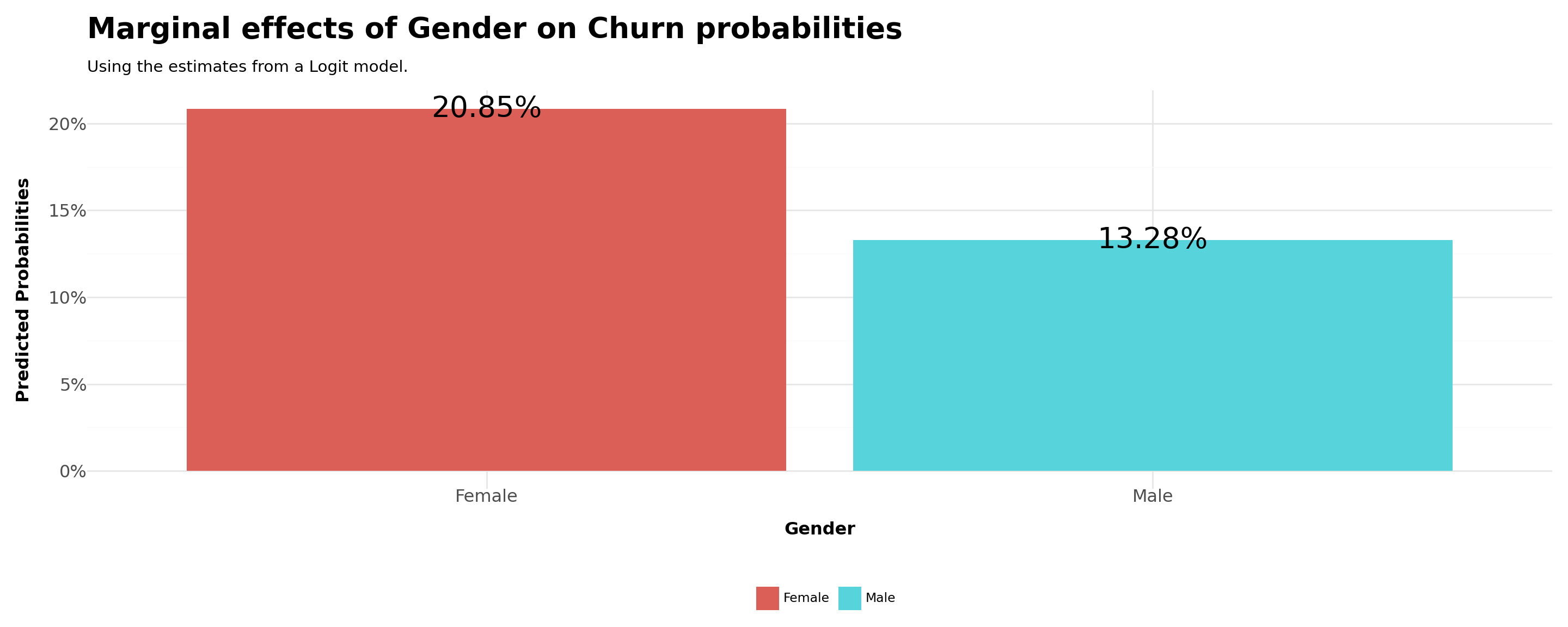
Another interesting use case is to re-do the same analysis before, but now varying also on categorical variables
For example, what is the difference in the probability of buying by men and women?
In order to do that, we can set all continous variables to their means and compare the estimated probabilities for
gender=1(male) andgender=0(female)
# Load data
data = pd.read_csv('Assets/bank-dataset.csv')
data['gender'] = np.where(data['gender'] == 'Male', 1, 0)

# Fit logistic regression model
X = data[['credit_score', 'age', 'tenure', 'balance', 'products_number', 'credit_card', 'active_member', 'estimated_salary','gender']]
X = sm.add_constant(X)  # Add constant term for intercept
y = data['churn']
model = sm.Logit(y, X).fit()

# Set all other variables to the mean
new_data = X.drop(columns=['gender']).mean(numeric_only=True).to_frame().transpose()
new_data = pd.DataFrame(np.repeat(new_data.values, 2, axis=0),columns=new_data.columns)
gender_df = pd.DataFrame(pd.Series(range(0, 2)), columns=['gender'])

# Concatenate with your existing DataFrame
concatenated_df = pd.concat([new_data, gender_df], ignore_index=True,axis=1)
concatenated_df.columns=[*new_data.columns,'gender']

# Predict on the new data
predicted_df = pd.DataFrame({
    'Gender': gender_df['gender'],
    'Predicted': model.predict(concatenated_df)
    })

predicted_df['Gender'] = np.where(concatenated_df['gender'] == 1, 'Male', 'Female')

# Plot
Plot = (
  ggplot(predicted_df,aes(x='Gender',y='Predicted',fill='Gender'))+
  geom_col()+
  geom_text(aes(label=predicted_df['Predicted']*100),format_string="{:.2f}%",size=20)+
  scale_y_continuous(labels = percent_format())+
  labs(
    title ='Marginal effects of Gender on Churn probabilities',
    subtitle = 'Using the estimates from a Logit model.',
    x = 'Gender',
    y = 'Predicted Probabilities',
    fill = '')+
  theme_minimal()+
  theme(
    legend_position='bottom',
    axis_title=element_text(face='bold',size=12),
    axis_text=element_text(size=12),
    plot_title=element_text(face='bold',size=20),
    figure_size=(15,6)
    )
  )

Plot.show()
Putting all together
We saw that women tend to churn, approximately, \(8\) percentage points more than men
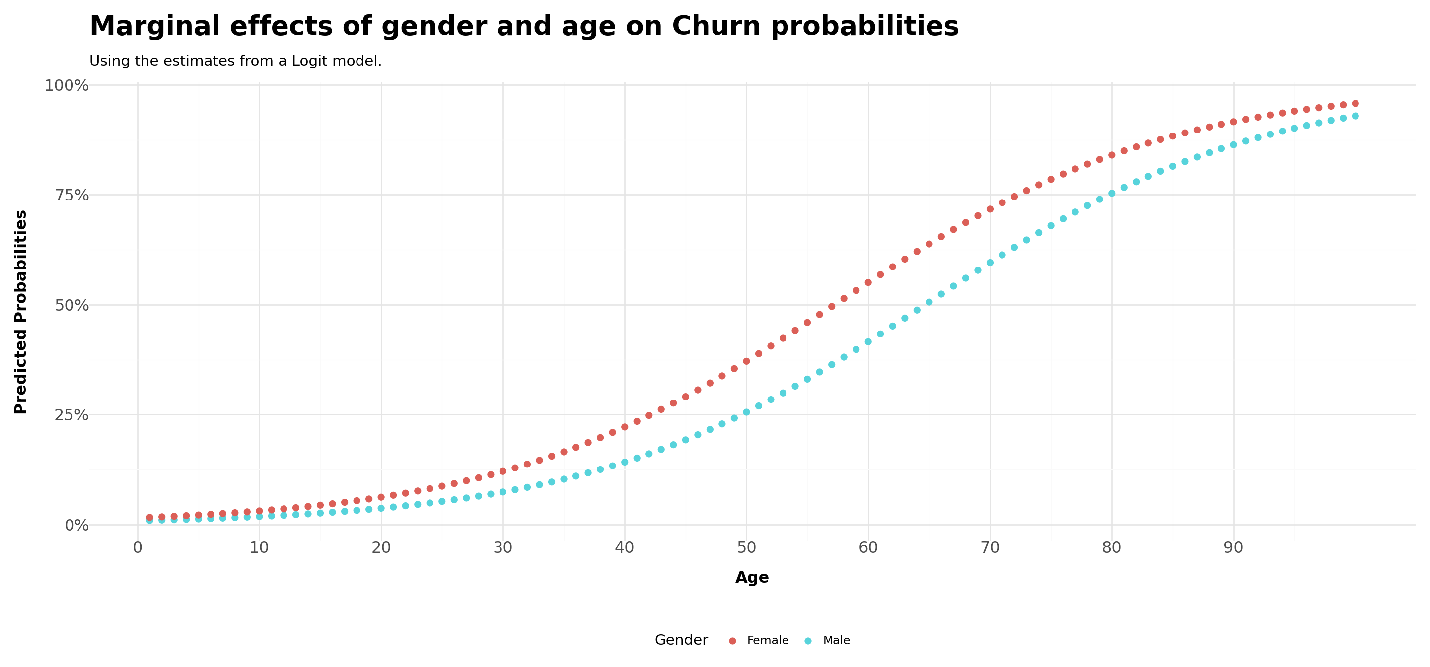
Is this true across all levels of age? As age levels increase, the gap between men and women may become wider due to personal traits. On the other hand, it may be that gender differences are invariant to age
In order to do that, we can do a mix of the two last exercises:
- Set all continuous variables, with the exception of
age, to their means - Compare the estimated probabilities for
gender=1(male) andgender=0(female) - You should have \(200\) rows in your data frame
# Load data
data = pd.read_csv('Assets/bank-dataset.csv')
data['gender'] = np.where(data['gender'] == 'Male', 1, 0)

# Fit logistic regression model
X = data[['credit_score', 'tenure', 'balance', 'products_number', 'credit_card', 'active_member', 'estimated_salary','gender','age']]
X = sm.add_constant(X)  # Add constant term for intercept
y = data['churn']
model = sm.Logit(y, X).fit()

# Set all other variables to the mean
new_data = X.drop(columns=['gender','age']).mean(numeric_only=True).to_frame().transpose()
new_data = pd.DataFrame(np.repeat(new_data.values, 200, axis=0),columns=new_data.columns)
gender_df = pd.DataFrame([*np.repeat(1,100,axis=0),*np.repeat(0,100,axis=0)], columns=['gender'])
age_df = pd.DataFrame(pd.Series(range(1, 101)), columns=['age'])
age_df =pd.concat([age_df,age_df],ignore_index=True,axis=0)

# Concatenate with your existing DataFrame
concatenated_df = pd.concat([gender_df, age_df], ignore_index=True,axis=1)
concatenated_df = pd.concat([new_data,concatenated_df], ignore_index=True,axis=1)
concatenated_df.columns=[*new_data.columns,'gender','age']

# Predict
predicted = model.predict(concatenated_df)
concatenated_df['Predicted'] = predicted
concatenated_df['Gender'] = np.where(concatenated_df['gender'] == 1, 'Male', 'Female')

# Plot
Plot = (
  ggplot(concatenated_df,aes(x='age',y='Predicted',fill='Gender'))+
  geom_point(stroke=0,size=3)+
  scale_y_continuous(labels = percent_format())+
  scale_x_continuous(breaks = range(0,100,10))+
  labs(
    title ='Marginal effects of gender and age on Churn probabilities',
    subtitle = 'Using the estimates from a Logit model.',
    x = 'Age',
    y = 'Predicted Probabilities',
    fill = 'Gender')+
  theme_minimal()+
  theme(
    legend_position='bottom',
    axis_title=element_text(face='bold',size=12),
    axis_text=element_text(size=12),
    plot_title=element_text(face='bold',size=20),
    figure_size=(15,7)
    )
  )

Plot.show()
Comparison across LPM and Logit estimations
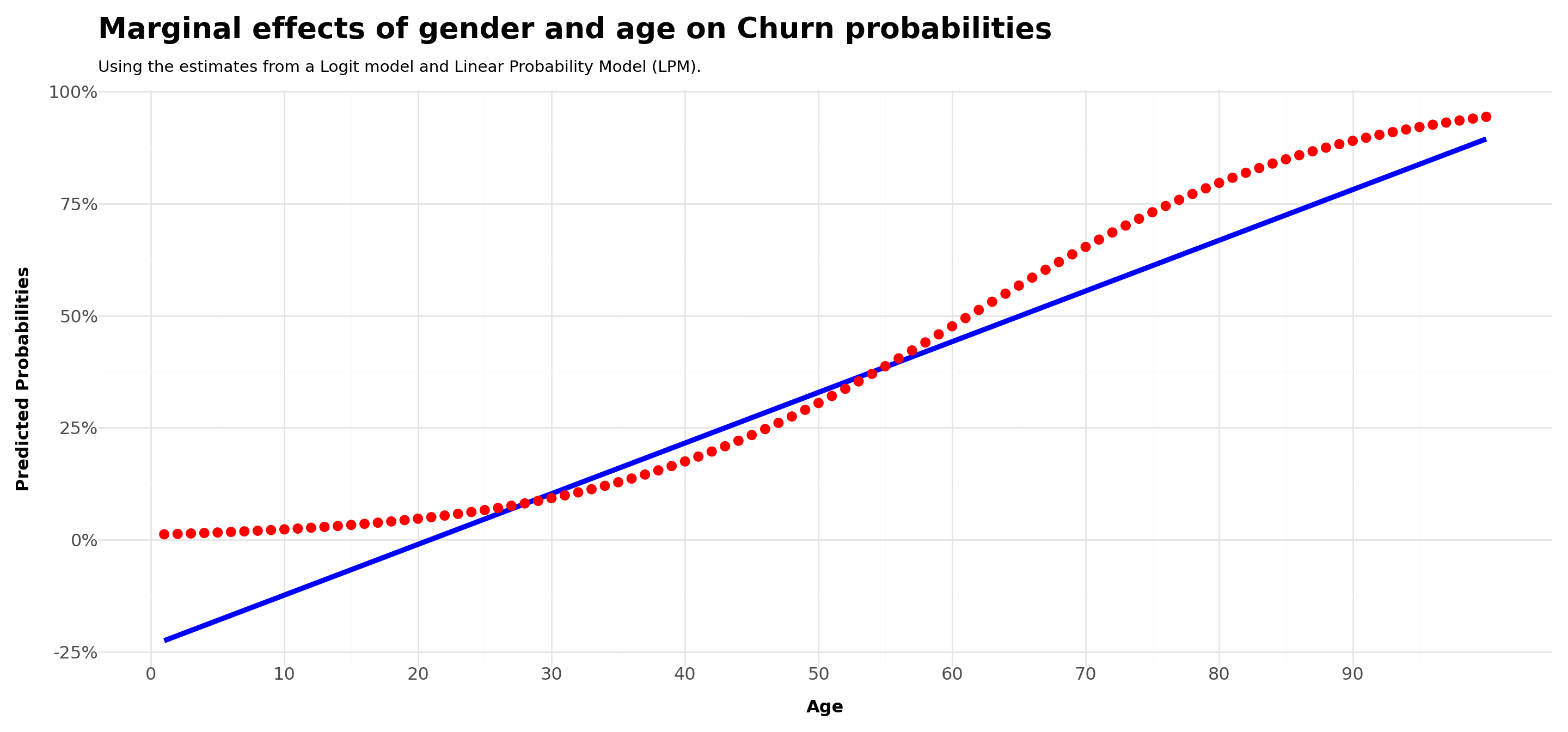
We came across two estimators for binary choice models. Do they differ in terms of the responses?
Although the coefficients from the different models are not directly comparable, we can use them to understand what are the partial effects:
For both cases, we’ll use all the other variables at their sample mean values:
- For LPM, the effect will be a slope, i.e., the marginal change depending on
Agewill be constant - For Logit, the change in the predicted probability will vary depending on the
Agereference point
- For LPM, the effect will be a slope, i.e., the marginal change depending on
Comparing across LPM and Logit estimations - age
# Read the CSV file into a pandas DataFrame
Data = pd.read_csv('Assets/bank-dataset.csv')

# Convert 'gender' into dummy variables
Data = pd.get_dummies(Data, columns=['gender'], drop_first=True)

# Define independent and dependent variables
X = Data[['credit_score', 'gender_Male', 'tenure', 'balance', 'products_number', 'credit_card', 'active_member', 'estimated_salary','age']]
y = Data['churn']

# Add a constant to the independent variables matrix for the intercept
X = sm.add_constant(X)

# Fit the linear regression model and the logit model
lm_model = sm.OLS(y, X.astype(float)).fit()
logit_model = sm.Logit(y, X.astype(float)).fit()

# Set all other variables to the mean
new_data = X.drop(columns=['age']).mean(numeric_only=True).to_frame().transpose()
new_data = pd.DataFrame(np.repeat(new_data.values, 100, axis=0),columns=new_data.columns)
age_df = pd.DataFrame(pd.Series(range(1, 101)), columns=['age'])

# Concatenate with your existing DataFrame
concatenated_df = pd.concat([new_data,age_df], ignore_index=True,axis=1)
concatenated_df.columns=[*new_data.columns,'age']

# Predict
lm_predicted = lm_model.predict(concatenated_df)
logit_predicted = logit_model.predict(concatenated_df)

predicted_df = pd.DataFrame({
  'LPM': lm_predicted,
  'Logit': logit_predicted,
  'Age': age_df['age']
})


# Plot
Plot = (
  ggplot(predicted_df,aes(x='Age'))+
  geom_line(aes(y='LPM'),color='blue',size=2)+
  geom_point(aes(y='Logit'),color='red',stroke=0,size=4)+
  scale_y_continuous(labels = percent_format())+
  scale_x_continuous(breaks = range(0,100,10))+
  labs(
    title ='Marginal effects of gender and age on Churn probabilities',
    subtitle = 'Using the estimates from a Logit model and Linear Probability Model (LPM).',
    x = 'Age',
    y = 'Predicted Probabilities',
    fill = 'Gender')+
  theme_minimal()+
  theme(
    legend_position='bottom',
    axis_title=element_text(face='bold',size=12),
    axis_text=element_text(size=12),
    plot_title=element_text(face='bold',size=20),
    figure_size=(15,7)
    )
  )

Plot.show()
Comparison across LPM and Logit estimations (continued)
In the LPM model, the effect of
ageis always the same – intuitively, \(\beta_{Age}\), the partial derivative of Y with respect toAge, is the same for all levelsOn the other hand, the changes when looking at the Logit model vary depending on the reference point for
Age:- For values \([0,20]\), it increases modestly
- Around \([21,60]\), the changes are exponential
- Between \([60,80]\), the changes start to become constant
- After 80, we see diminishing effects
Do these differences matter in practice? It depends on what you’re looking… (more on the next slide)
Comparison across LPM and Logit estimations (continued)
On the one hand, we clearly the weaknesses of the LPM when estimating probabilities for ages between \([0,20]\).
On the other hand, LPM and Logit will be almost identical between \([30,60]\)
If you tabulate the distribution of
Agein your dataset, you’ll see that although LPM does a poor job in predicting probabilities for cases \(<20\), the sample proportion of these cases is less than \(1\%\)On the other hand, its results are approximately the same as of Logit between \([30,60]\), which constitutes approximately \(80\%\) of the sample, which indicates that for the specific sample you are looking at, a LPM is not a terrible idea
Wrapping-up
Logit or LPM?
If your interest is to use the model results to predict probabilities for different age brackets, then yes, you should use Logit (or any model with the similar properties)
If, on the other hand, you’re just interest in knowing the effects for the average person in your sample (or extrapolating a causal effect if applicable), you can use LPM
Strengths and weaknesses
LPM is simpler, and we know very well the properties to analyze cases potential issues such as ommited variable bias
In the Logit world, there is no \(R^2\), but there are other ways to check the predictive ability and fit of models
\(\rightarrow\) In our next lecture, we will understand how to evaluate Logit models using metrics that are more suitable for the task!
